-
.NET (.NET Core)
-
1C
-
APL
-
AWK
-
Agda
-
Agile/Scrum
-
Alef
-
Assembler
-
Basic
-
Beta Programming Language
-
Big Data/DataScience
-
C
-
C#
-
C++
-
CSS
-
Cobol
-
Crystal
-
D
-
Dart
-
DataBase (SQL)
-
Delphi
-
F#
-
Flutter
-
Fortran
-
GPT/AI/ИИ
-
GameDev
-
Git
-
Go (Golang)
-
HTML
-
Hacking and Security
-
Haskell
-
Java
-
JavaScript (JS)
-
Julia
-
Kotlin
-
Machine Learning (ML)
-
Natural language processing (NLP)
-
PHP
-
Pascal
-
Python
-
R
-
Ruby
-
Rust
-
Scratch
-
Swift
-
UML
-
UX/UI
-
Visual Basic
-
Wolfram
-
XML
-
АСУ
-
Проектирование/System Design
-
Сети/Network
-
Схемотехника/электронные схемы
-
.NET (.NET Core)
-
1C
-
APL
-
AWK
-
Agda
-
Agile/Scrum
-
Alef
-
Assembler
-
Basic
-
Beta Programming Language
-
Big Data/DataScience
-
C
-
C#
-
C++
-
CSS
-
Cobol
-
Crystal
-
D
-
Dart
-
DataBase (SQL)
-
Delphi
-
F#
-
Flutter
-
Fortran
-
GPT/AI/ИИ
-
GameDev
-
Git
-
Go (Golang)
-
HTML
-
Hacking and Security
-
Haskell
-
Java
-
JavaScript (JS)
-
Julia
-
Kotlin
-
Machine Learning (ML)
-
Natural language processing (NLP)
-
PHP
-
Pascal
-
Python
-
R
-
Ruby
-
Rust
-
Scratch
-
Swift
-
UML
-
UX/UI
-
Visual Basic
-
Wolfram
-
XML
-
АСУ
-
Проектирование/System Design
-
Сети/Network
-
Схемотехника/электронные схемы
Меню
Statistics Slam Dunk: Statistical analysis with R on real NBA data
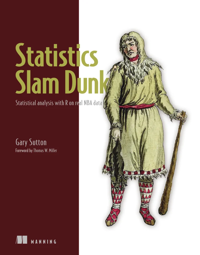
Автор: Sutton Gary
Дата выхода: 2024
Издательство: Manning Publications Co.
Количество страниц: 672
Размер файла: 7,0 МБ
Тип файла: PDF
Добавил: codelibs
Statistics Slam Dunk....1
brief contents....8
contents....10
foreword....17
preface....19
acknowledgments....21
about this book....23
Who should read this book....23
How this book is organized: A road map....24
About the code....27
liveBook discussion forum....27
about the author....28
about the cover illustration....29
Chapter 1: Getting started....31
1.1 Brief introductions to R and RStudio....32
1.2 Why R?....34
1.2.1 Visualizing data....34
1.2.2 Installing and using packages to extend R’s functional footprint....37
1.2.3 Networking with other users....38
1.2.4 Interacting with big data....39
1.2.5 Landing a job....39
1.3 How this book works....39
Chapter 2: Exploring data....44
2.1 Loading packages....45
2.2 Importing data....46
2.3 Wrangling data....47
2.3.1 Removing variables....48
2.3.2 Removing observations....48
2.3.3 Viewing data....49
2.3.4 Converting variable types....50
2.3.5 Creating derived variables....51
2.4 Variable breakdown....53
2.5 Exploratory data analysis....55
2.5.1 Computing basic statistics....55
2.5.2 Returning data....58
2.5.3 Computing and visualizing frequency distributions....59
2.5.4 Computing and visualizing correlations....72
2.5.5 Computing and visualizing means and medians....75
2.6 Writing data....81
Chapter 3: Segmentation analysis....83
3.1 More on tanking and the draft....84
3.2 Loading packages....85
3.3 Importing and viewing data....86
3.4 Creating another derived variable....87
3.5 Visualizing means and medians....88
3.5.1 Regular season games played....88
3.5.2 Minutes played per game....92
3.5.3 Career win shares....94
3.5.4 Win shares every 48 minutes....96
3.6 Preliminary conclusions....98
3.7 Sankey diagram....99
3.8 Expected value analysis....104
3.9 Hierarchical clustering....110
Chapter 4: Constrained optimization....116
4.1 What is constrained optimization?....117
4.2 Loading packages....118
4.3 Importing data....119
4.4 Knowing the data....119
4.5 Visualizing the data....122
4.5.1 Density plots....122
4.5.2 Boxplots....125
4.5.3 Correlation plot....127
4.5.4 Bar chart....129
4.6 Constrained optimization setup....132
4.7 Constrained optimization construction....134
4.8 Results....139
Chapter 5: Regression models....142
5.1 Loading packages....144
5.2 Importing data....144
5.3 Knowing the data....145
5.4 Identifying outliers....148
5.4.1 Prototype....148
5.4.2 Identifying other outliers....152
5.5 Checking for normality....157
5.5.1 Prototype....158
5.5.2 Checking other distributions for normality....159
5.6 Visualizing and testing correlations....163
5.6.1 Prototype....164
5.6.2 Visualizing and testing other correlations....165
5.7 Multiple linear regression....167
5.7.1 Subsetting data into train and test....167
5.7.2 Fitting the model....168
5.7.3 Returning and interpreting the results....168
5.7.4 Checking for multicollinearity....171
5.7.5 Running and interpreting model diagnostics....172
5.7.6 Comparing models....173
5.7.7 Predicting....176
5.8 Regression tree....180
Chapter 6: More wrangling and visualizing data....184
6.1 Loading packages....185
6.2 Importing data....185
6.3 Wrangling data....186
6.3.1 Subsetting data sets....186
6.3.2 Joining data sets....187
6.4 Analysis....191
6.4.1 First quarter....191
6.4.2 Second quarter....195
6.4.3 Third quarter....198
6.4.4 Fourth quarter....199
6.4.5 Comparing best and worst teams....201
6.4.6 Second-half results....211
Chapter 7: T-testing and effect size testing....217
7.1 Loading packages....218
7.2 Importing data....219
7.3 Wrangling data....219
7.4 Analysis on 2018–19 data....221
7.4.1 2018–19 regular season analysis....221
7.4.2 2019 postseason analysis....227
7.4.3 Effect size testing....231
7.5 Analysis on 2019–20 data....233
7.5.1 2019–20 regular season analysis (pre-COVID)....233
7.5.2 2019–20 regular season analysis (post-COVID)....238
7.5.3 More effect size testing....241
Chapter 8: Optimal stopping....244
8.1 Loading packages....245
8.2 Importing images....245
8.3 Importing and viewing data....246
8.4 Exploring and wrangling data....247
8.5 Analysis....252
8.5.1 Milwaukee Bucks....252
8.5.2 Atlanta Hawks....259
8.5.3 Charlotte Hornets....263
8.5.4 NBA....267
Chapter 9: Chi-square testing and more effect size testing....271
9.1 Loading packages....272
9.2 Importing data....273
9.3 Wrangling data....274
9.4 Computing permutations....277
9.5 Visualizing results....279
9.5.1 Creating a data source....280
9.5.2 Visualizing the results....281
9.5.3 Conclusions....283
9.6 Statistical test of significance....285
9.6.1 Creating a contingency table and a balloon plot....286
9.6.2 Running a chi-square test....288
9.6.3 Creating a mosaic plot....288
9.7 Effect size testing....289
Chapter 10: Doing more with ggplot2....291
10.1 Loading packages....292
10.2 Importing and viewing data....292
10.3 Salaries and salary cap analysis....294
10.4 Analysis....300
10.4.1 Plotting and computing correlations between team payrolls and regular season wins....301
10.4.2 Payrolls versus end-of-season results....312
10.4.3 Payroll comparisons....315
Chapter 11: K-means clustering....323
11.1 Loading packages....324
11.2 Importing data....324
11.3 A primer on standard deviations and z-scores....325
11.4 Analysis....327
11.4.1 Wrangling data....328
11.4.2 Evaluating payrolls and wins....332
11.5 K-means clustering....337
11.5.1 More data wrangling....339
11.5.2 K-means clustering....341
Chapter 12: Computing and plotting inequality....352
12.1 Gini coefficients and Lorenz curves....353
12.2 Loading packages....354
12.3 Importing and viewing data....355
12.4 Wrangling data....357
12.5 Gini coefficients....363
12.6 Lorenz curves....367
12.7 Salary inequality and championships....371
12.7.1 Wrangling data....372
12.7.2 T-test....376
12.7.3 Effect size testing....379
12.8 Salary inequality and wins and losses....380
12.8.1 T-test....380
12.8.2 Effect size testing....382
12.9 Gini coefficient bands versus winning percentage....383
Chapter 13: More with Gini coefficients and Lorenz curves....388
13.1 Loading packages....389
13.2 Importing and viewing data....390
13.3 Wrangling data....390
13.4 Gini coefficients....396
13.5 Lorenz curves....399
13.6 For loops....403
13.6.1 Simple demonstration....404
13.6.2 Applying what we’ve learned....404
13.7 User-defined functions....408
13.8 Win share inequality and championships....411
13.8.1 Wrangling data....412
13.8.2 T-test....417
13.8.3 Effect size testing....420
13.9 Win share inequality and wins and losses....423
13.9.1 T-test....423
13.9.2 Effect size testing....426
13.10 Gini coefficient bands versus winning percentage....426
Chapter 14: Intermediate and advanced modeling....431
14.1 Loading packages....432
14.2 Importing and wrangling data....432
14.2.1 Subsetting and reshaping our data....433
14.2.2 Extracting a substring to create a new variable....435
14.2.3 Joining data....436
14.2.4 Importing and wrangling additional data sets....436
14.2.5 Joining data (one more time)....439
14.2.6 Creating standardized variables....440
14.3 Exploring data....441
14.4 Correlations....445
14.4.1 Computing and plotting correlation coefficients....445
14.4.2 Running correlation tests....449
14.5 Analysis of variance models....450
14.5.1 Data wrangling and data visualization....451
14.5.2 One-way ANOVAs....454
14.6 Logistic regressions....458
14.6.1 Data wrangling....459
14.6.2 Model development....460
14.7 Paired data before and after....471
Chapter 15: The Lindy effect....477
15.1 Loading packages....479
15.2 Importing and viewing data....479
15.3 Visualizing data....482
15.3.1 Creating and evaluating violin plots....483
15.3.2 Creating paired histograms....484
15.3.3 Printing our plots....485
15.4 Pareto charts....487
15.4.1 ggplot2 and ggQC packages....488
15.4.2 qcc package....490
Chapter 16: Randomness versus causality....494
16.1 Loading packages....495
16.2 Importing and wrangling data....496
16.3 Rule of succession and the hot hand....498
16.4 Player-level analysis....503
16.4.1 Player 1 of 3: Giannis Antetokounmpo....503
16.4.2 Player 2 of 3: Julius Randle....508
16.4.3 Player 3 of 3: James Harden....512
16.5 League-wide analysis....515
Chapter 17: Collective intelligence....520
17.1 Loading packages....521
17.2 Importing data....522
17.3 Wrangling data....522
17.4 Automated exploratory data analysis....526
17.4.1 Baseline EDA with tableone....526
17.4.2 Over/under EDA with DataExplorer....529
17.4.3 Point spread EDA with SmartEDA....543
17.5 Results....552
17.5.1 Over/under....553
17.5.2 Point spreads....564
Chapter 18: Statistical dispersion methods....570
18.1 Loading a package....571
18.2 Importing data....571
18.3 Exploring and wrangling data....572
18.4 Measures of statistical dispersion and intra-season parity....576
18.4.1 Variance method....576
18.4.2 Standard deviation method....579
18.4.3 Range method....581
18.4.4 Mean absolute deviation method....583
18.4.5 Median absolute deviation method....586
18.5 Churn and inter-season parity....588
18.5.1 Data wrangling....589
18.5.2 Computing and visualizing churn....590
Chapter 19: Data standardization....595
19.1 Loading a package....596
19.2 Importing and viewing data....597
19.3 Wrangling data....598
19.3.1 Treating duplicate records....598
19.3.2 Final trimmings....602
19.4 Standardizing data....603
19.4.1 Z-score method....605
19.4.2 Standard deviation method....608
19.4.3 Centering method....610
19.4.4 Range method....612
Chapter 20: Finishing up....616
20.1 Cluster analysis....617
20.2 Significance testing....619
20.3 Effect size testing....622
20.4 Modeling....624
20.5 Operations research....627
20.6 Probability....630
20.7 Statistical dispersion....632
20.8 Standardization....633
20.9 Summary statistics and visualization....635
Appendix: More ggplot2 visualizations....639
index....661
Numerics....661
A....661
B....661
C....661
D....662
E....664
F....664
G....664
H....665
I....665
J....665
K....665
L....666
M....666
N....667
O....667
P....667
Q....668
R....668
S....668
T....669
U....670
V....670
W....670
X....670
Y....670
Z....670
Statistics Slam Dunk is a data science manual with a difference. Each chapter is a complete, self-contained statistics or data science project for you to work through—from importing data, to wrangling it, testing it, visualizing it, and modeling it. Throughout the book, you’ll work exclusively with NBA data sets and the R language, applying best-in-class statistics techniques to reveal fun and fascinating truths about the NBA.
About the book
Is losing basketball games on purpose a rational strategy? Which hustle statistics have an impact on wins and losses? Does spending more on player salaries translate into a winning record? You’ll answer all these questions and more. Plus, R’s visualization capabilities shine through in the book’s 300 plots and charts, including Pareto charts, Sankey diagrams, Cleveland dot plots, and dendrograms.
What's inside
- Transforming, tidying, and wrangling data
- Applying best-in-class exploratory data analysis techniques
- Developing supervised and unsupervised machine learning algorithms
- Executing hypothesis tests and effect size tests
About the reader
For readers who know basic statistics. No advanced knowledge of R—or basketball—required.
